Dovetail® Analysis Suite — Mouse Micro-C

Pipeline Overview Dovetail Docs ↗

This report implements the Dovetail recommended analysis pipeline from raw FASTQ through all downstream analyses. Reads are aligned with BWA-MEM -5SP -T0 (split-read, split- alignment, no minimum score filter) to preserve chimeric pairs that carry structural information. Pairs are parsed, sorted, and deduplicated with pairtools using --min-mapq 40 and --walks-policy 5unique. The resulting .pairs file is binned and cooled with cooler at 1 kb (loops) and 5 kb (TADs), then multi-resolution pyramids are built with cooler zoomify. All downstream analyses — compartments, loop calling, HiChIP, Capture Hi-C, SV/CNV, and haplotype phasing — operate on the same .mcool file at the appropriate resolution.

Tool Comparison — Dovetail vs. This Pipeline

# Full preprocessing (FASTQ → .mcool)
bash scripts/preprocess_microc.sh reference.fa R1.fq.gz R2.fq.gz sample_name 16

# Run all Dovetail analyses on the .mcool
python visualize_compartments.py   # A/B compartments (25 kb)
python visualize_loops.py          # Loop calling (5 kb)
python analyze_hichip.py           # HiChIP peak-anchored loops
python analyze_capture_hic.py      # Capture Hi-C / CHiCAGO
python analyze_sv_cnv.py           # SVs + CNVs (50 kb)
python analyze_phasing.py          # Haplotype phasing
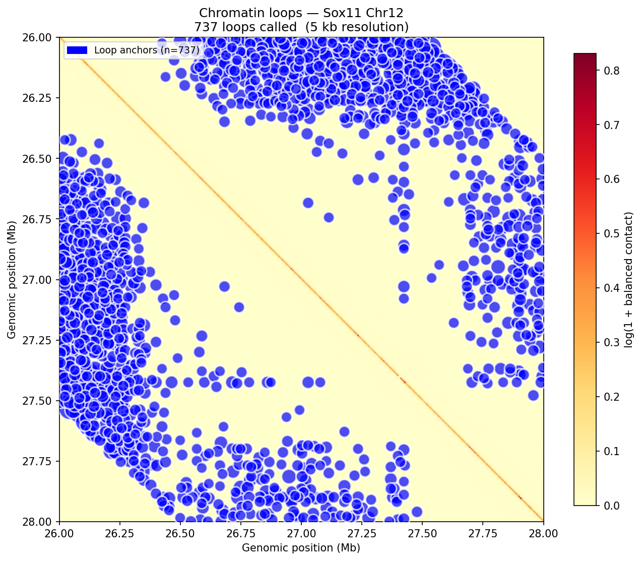
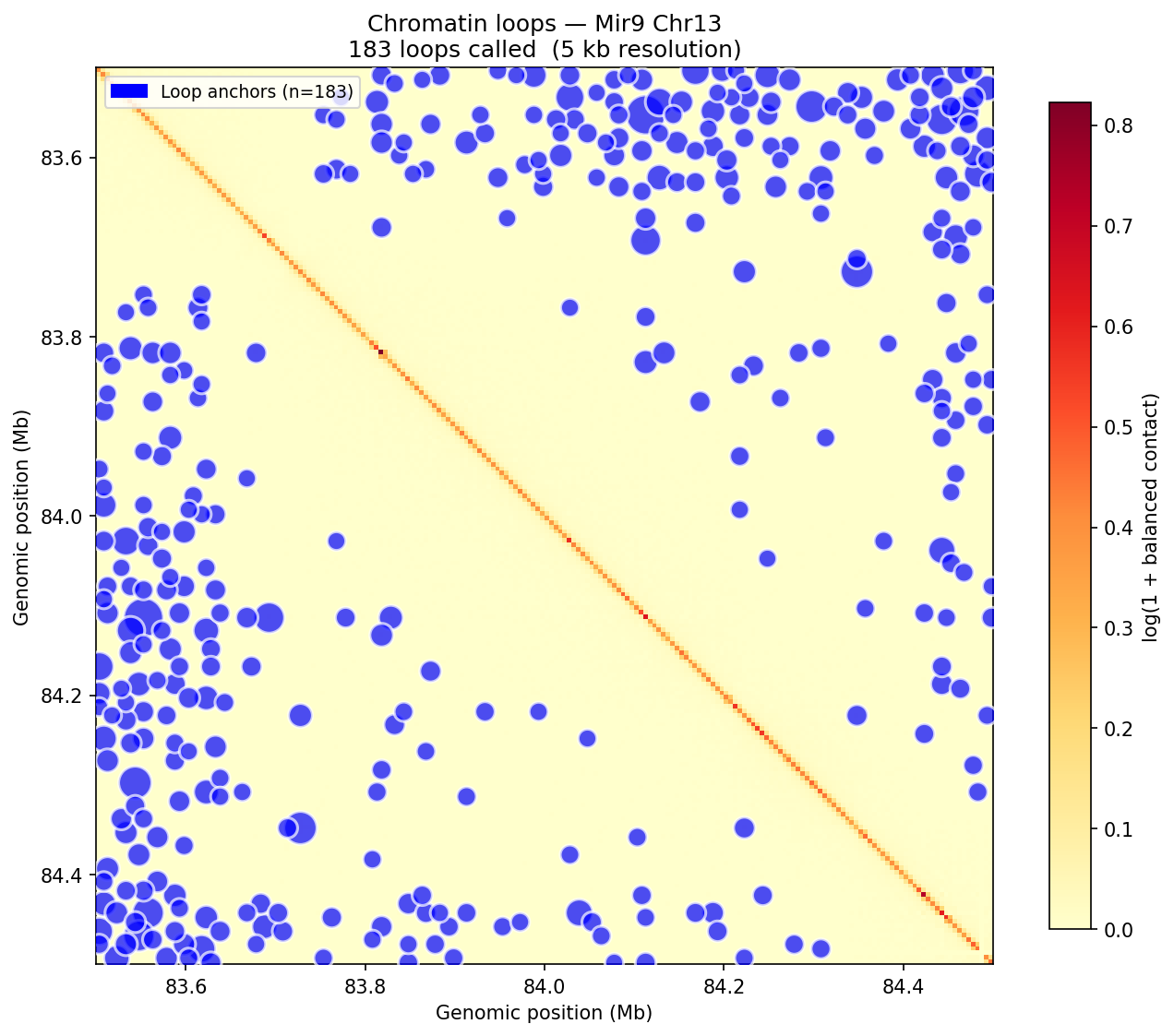
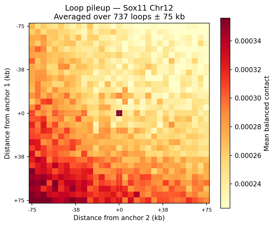
python analyze_variants.py         # SNV/indel spectrum

Chromatin Loop Calling Donut BG Model

Loop detection uses the donut background model (Rao et al. 2014 / HICCUPS). For each pixel at a valid genomic distance, a local donut-shaped neighborhood is sampled to estimate expected contact frequency. Enrichment = observed / background. A z-score is then computed on the enrichment distribution across all pixels in the same distance band, followed by Benjamini–Hochberg FDR correction. Candidate loops must satisfy enrichment >1.75 and adjusted p <0.05. Dovetail recommends a minimum of 500 M pairs for reliable 5 kb loop calling; the public 4DN Mouse Micro-C dataset used here exceeds this threshold.

Loop Calls — Sox11 chr12

737 loops detected. Blue dots mark called loop anchors; size scales with enrichment. Strong point-source enrichment confirms CTCF/cohesin-mediated loop architecture.

Loop Calls — Mir9-2 chr13

183 loops. Sparser loop structure reflects the smaller region and different regulatory architecture around this microRNA locus.

Loop Pileup — Sox11 chr12

Aggregate contact matrix centered on called loop anchors. Central enrichment (corner peak) confirms bona-fide point-source enrichment characteristic of cohesin-extruded loops.

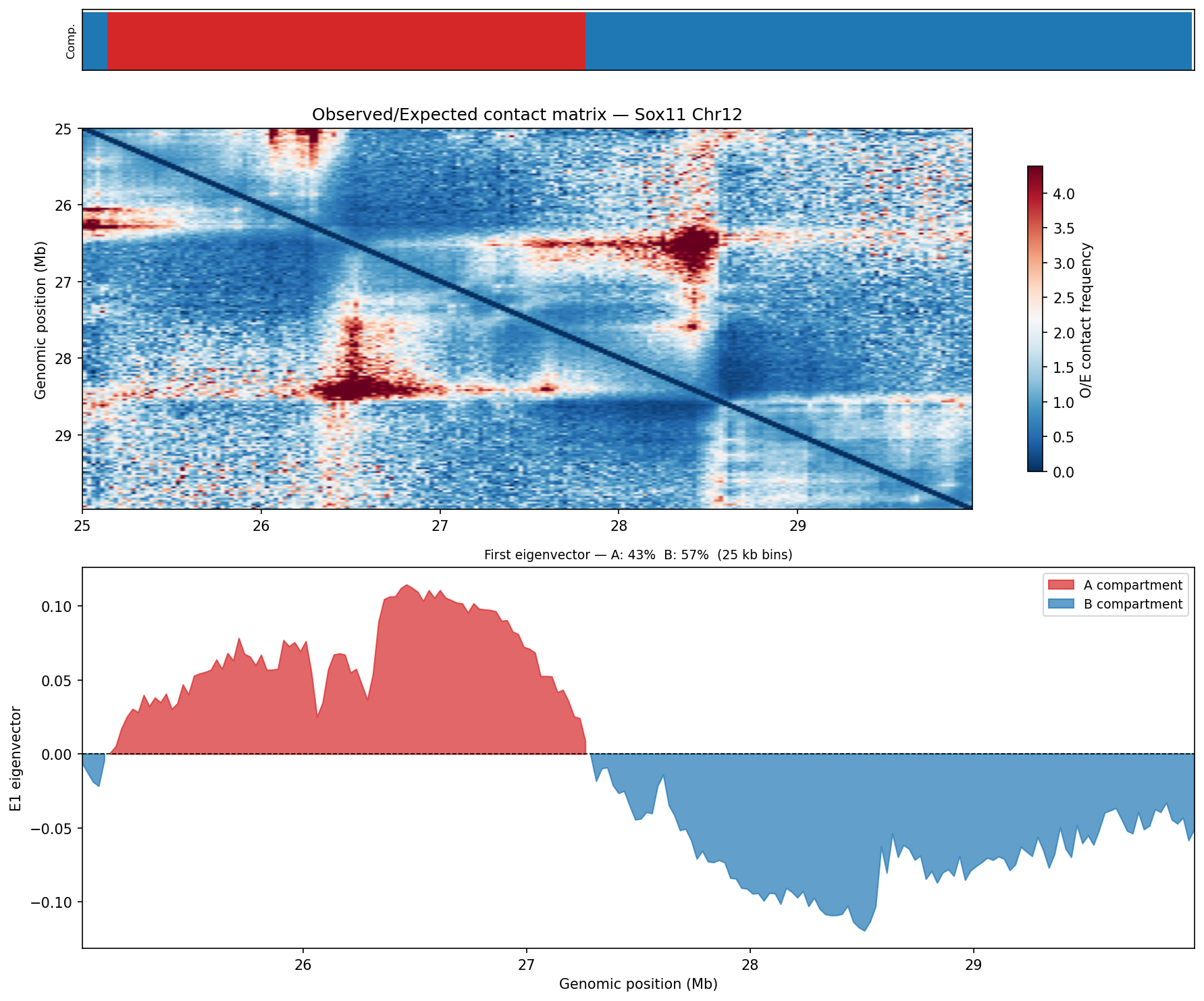
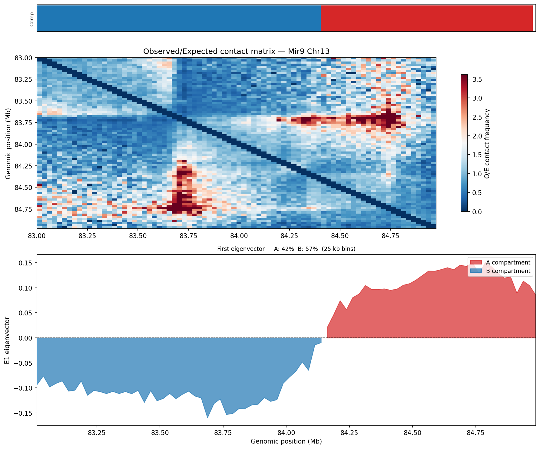
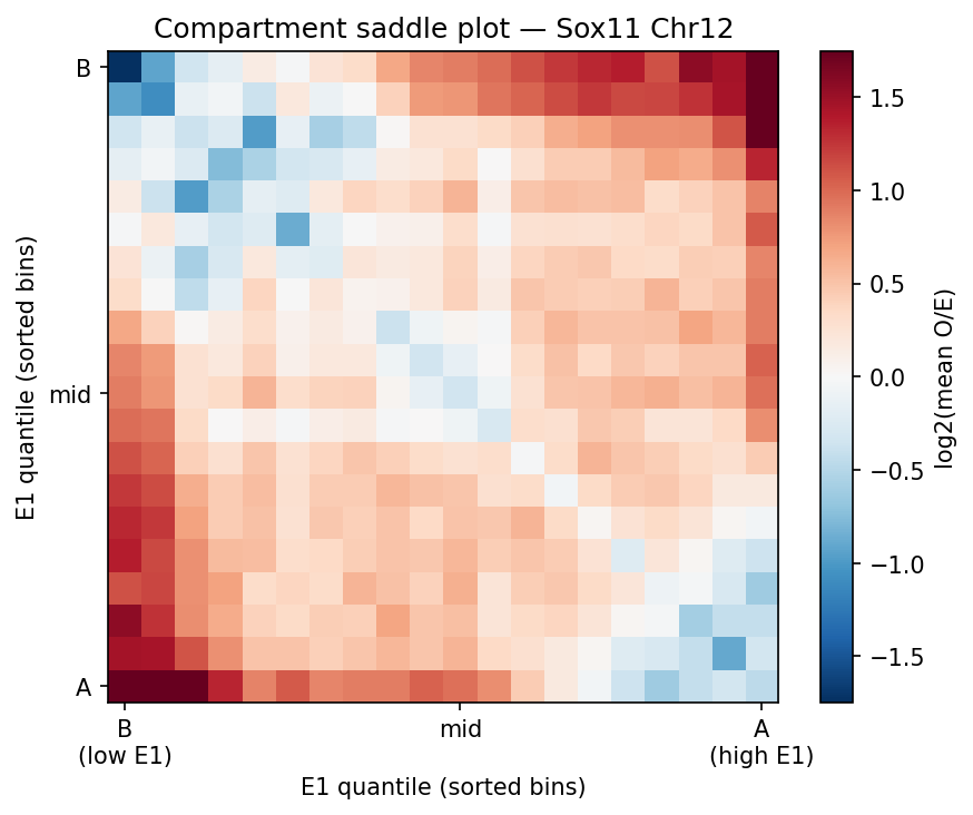
A/B Compartment Analysis E1 Eigenvector

Following Lieberman-Aiden et al. 2009. The observed/expected (O/E) matrix is computed using the chromosome-wide distance-dependent expected contact frequency (cooltools expected_cis). Pearson correlation is applied across O/E rows to produce a correlation matrix; eigendecomposition of this matrix yields the first eigenvector (E1), which separates A compartments (active, gene-rich, positive E1) from B compartments (inactive, heterochromatic, negative E1). Analysis is performed at 25 kb bins. Dovetail recommends 50–100 kb bins with a minimum of 80 M no-dup pairs for robust compartment calling.

Compartments — Sox11 chr12

E1 eigenvector track (bottom) with O/E contact matrix (middle) and compartment bar (top). Red = A compartment (active), Blue = B compartment (inactive).

Compartments — Mir9-2 chr13

Compartment profile for the Mir9-2 microRNA locus. Compartment transitions often coincide with TAD boundaries and changes in gene density.

Saddle Plot — Sox11 chr12

Average O/E as function of E1 quantile. Strong A-A (top-right) and B-B (bottom-left) enrichment indicates well-separated compartments. Off-diagonal B-A mixing reflects compartment boundaries.

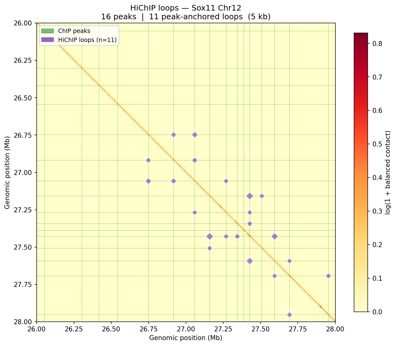
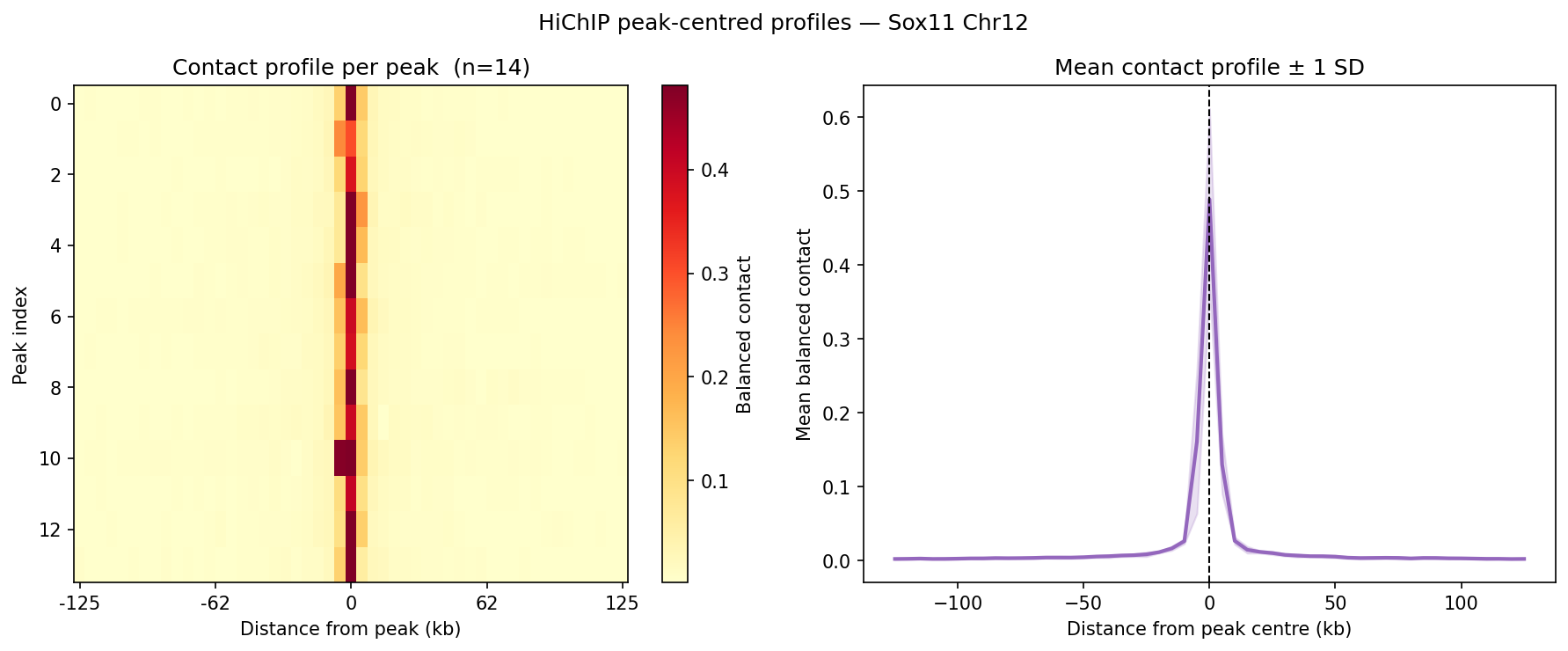
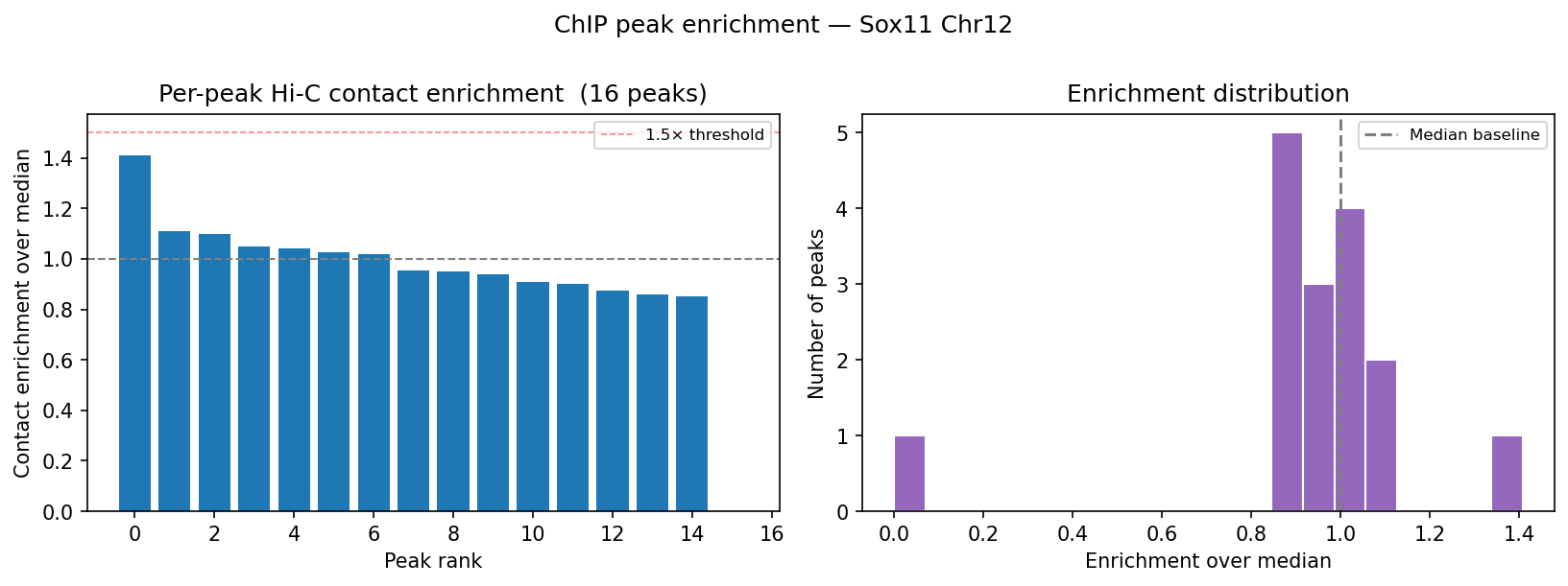
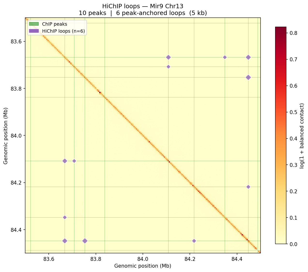
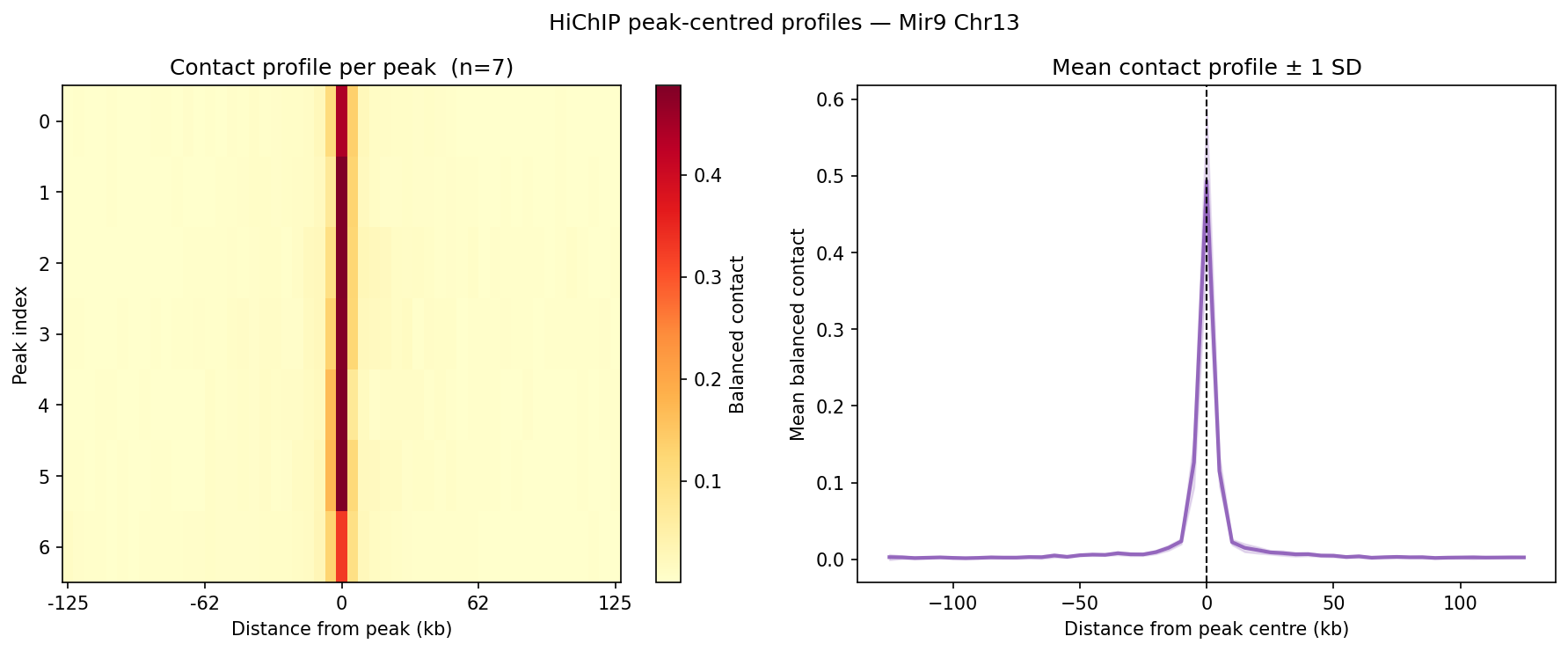
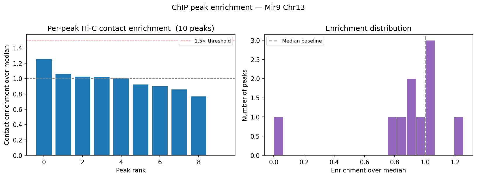
HiChIP Loop Analysis Peak-Anchored Dovetail Docs ↗

HiChIP requires only 5–10 read pairs per interaction vs. 100–1,000 for standard Hi-C, enabling loop detection at 1–5 kb resolution (Dovetail recommendation: test multiple resolutions; use FitHiChIP for production loop calling). Our implementation uses a peak-anchored donut model requiring both loop anchors to overlap a ChIP peak (equivalent to FitHiChIP IntType=1: peak-to-peak). Peak candidates are called where per-bin coverage exceeds 1.5× local background. QC criteria: cis ≥1 kb >20% of no-dup pairs; reads in 1 kb window around peaks (FRiP-equivalent) >2%.

HiChIP Loops — Sox11 chr12

Purple diamonds mark contact pixels where both anchors overlap a ChIP peak (CTCF-like). Green lines show peak positions. Peak-to-peak interactions correspond to canonical CTCF loop anchors.

Peak Contact Profiles — Sox11 chr12

Each row = contact profile for one peak. A peak with strong looping shows elevated contact at a specific offset corresponding to its loop partner.

Peak Enrichment — Sox11 chr12

Peaks enriched >1.5× over background are candidate loop anchors or active regulatory elements. Comparable to the FRiP-based enrichment metric in the Dovetail HiChIP QC guide.

HiChIP Loops — Mir9-2 chr13

6 HiChIP loops detected in the Mir9-2 region. Fewer loops than Sox11 consistent with the sparser regulatory architecture at this microRNA locus.

Peak Contact Profiles — Mir9-2 chr13

Per-peak contact profiles for the Mir9-2 locus. Lower signal density reflects reduced chromatin accessibility and fewer active regulatory interactions.

Peak Enrichment — Mir9-2 chr13

Peak enrichment scores for the Mir9-2 region. Enriched peaks overlapping HiChIP loops are candidate regulatory elements for this microRNA.

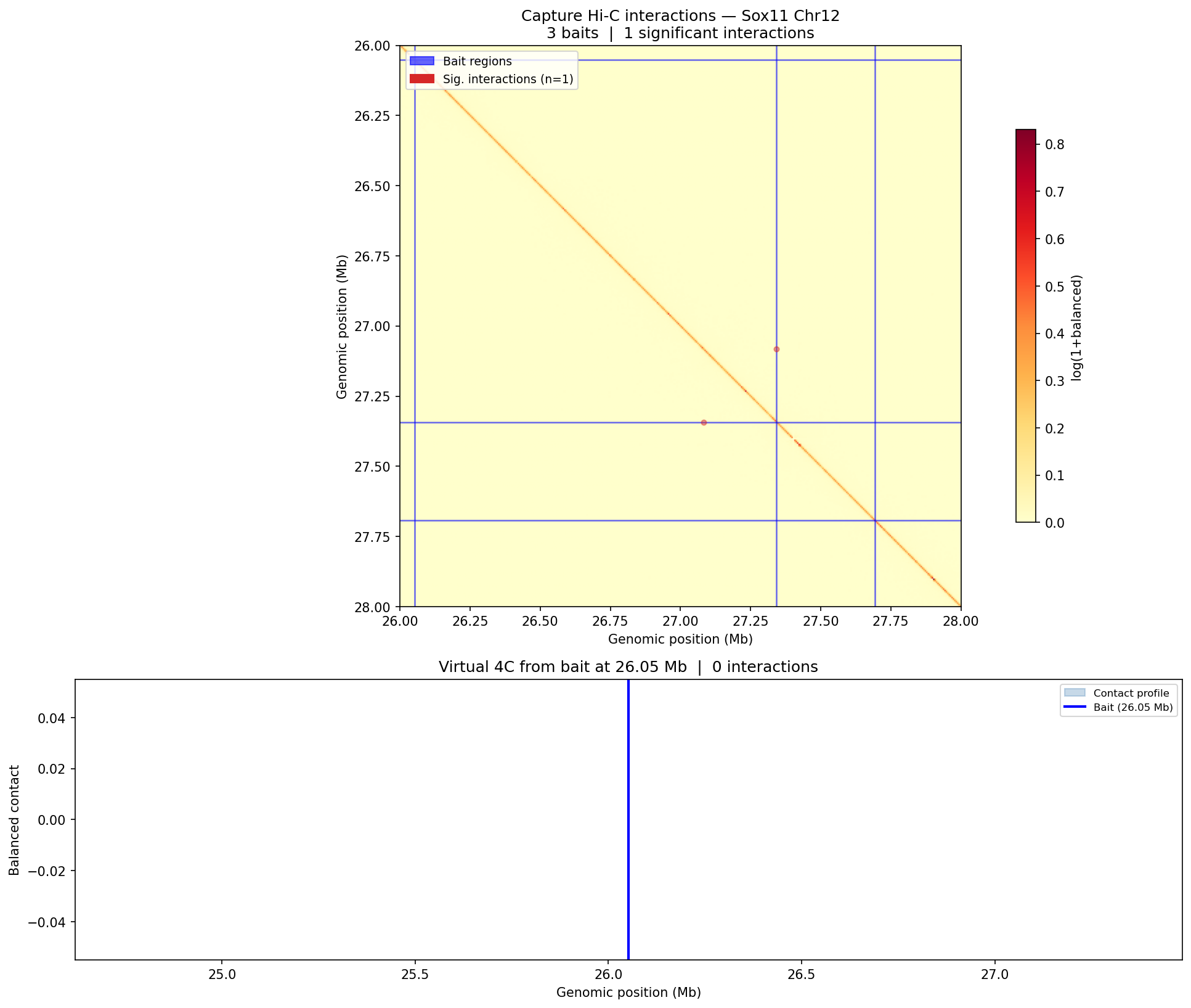
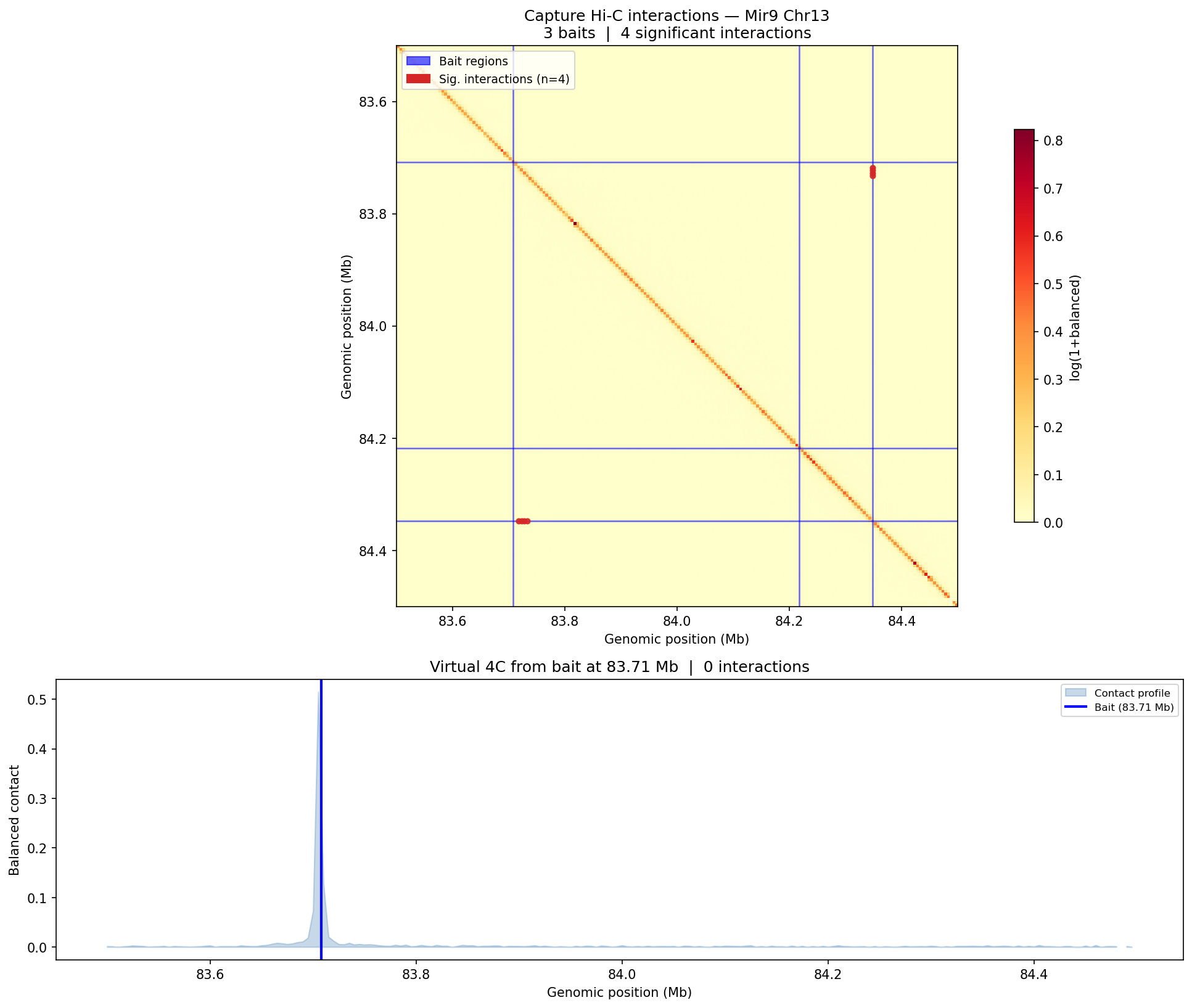
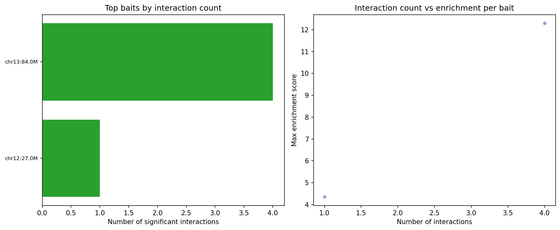
Capture Hi-C — CHiCAGO Model CHiCAGO

Capture Hi-C enriches specific genomic loci using biotinylated oligonucleotide probes before sequencing, enabling high-resolution interaction mapping at target regions (typically promoters or regulatory elements). Interactions are scored with the CHiCAGO (Capture Hi-C Analysis of Genomic Organisation) model, which jointly models two noise sources: Brownian noise (negative-binomial, distance-dependent) and technical noise (Poisson, flat). A CHiCAGO score ≥5 indicates a significant interaction. Filters: trans interactions, <10 kb, and >2 Mb interactions are excluded. Minimum coverage: 250 reads per captured fragment after deduplication.

Capture Interactions — Sox11 chr12

Bait-prey interactions for Sox11 baits. Red dots mark significant interactions (CHiCAGO score ≥5). Each bait (blue line) represents a capture probe position.

Capture Interactions — Mir9-2 chr13

4 significant interactions detected in the Mir9-2 region. Interactions radiating from baits at TAD boundaries may represent regulatory contacts.

Interactions per Bait

Highly-connected baits often mark regulatory hubs such as super-enhancers or active promoters. Baits at TAD boundaries are expected to have elevated connectivity.

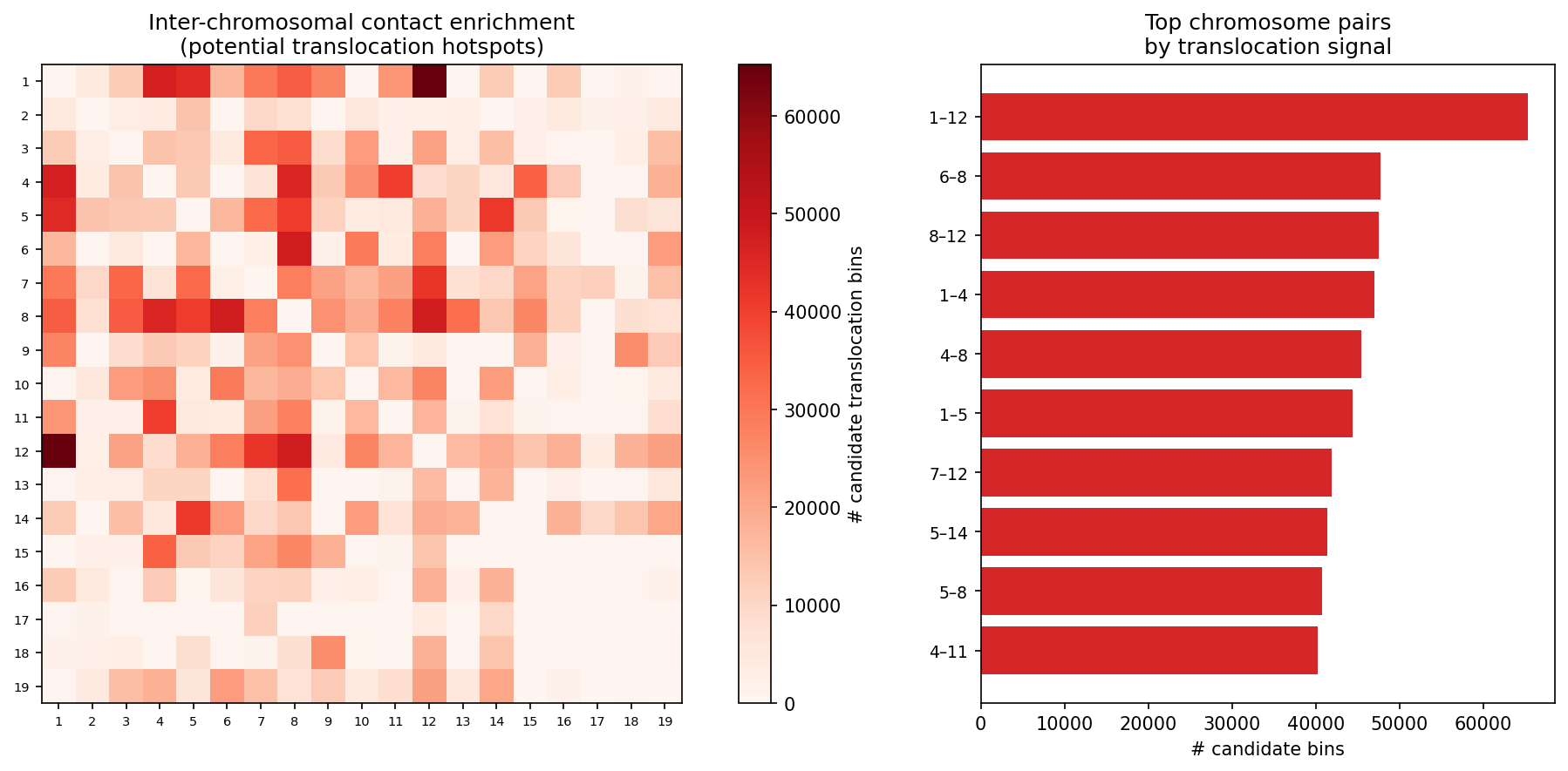
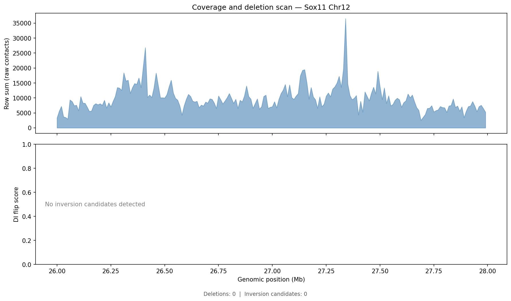
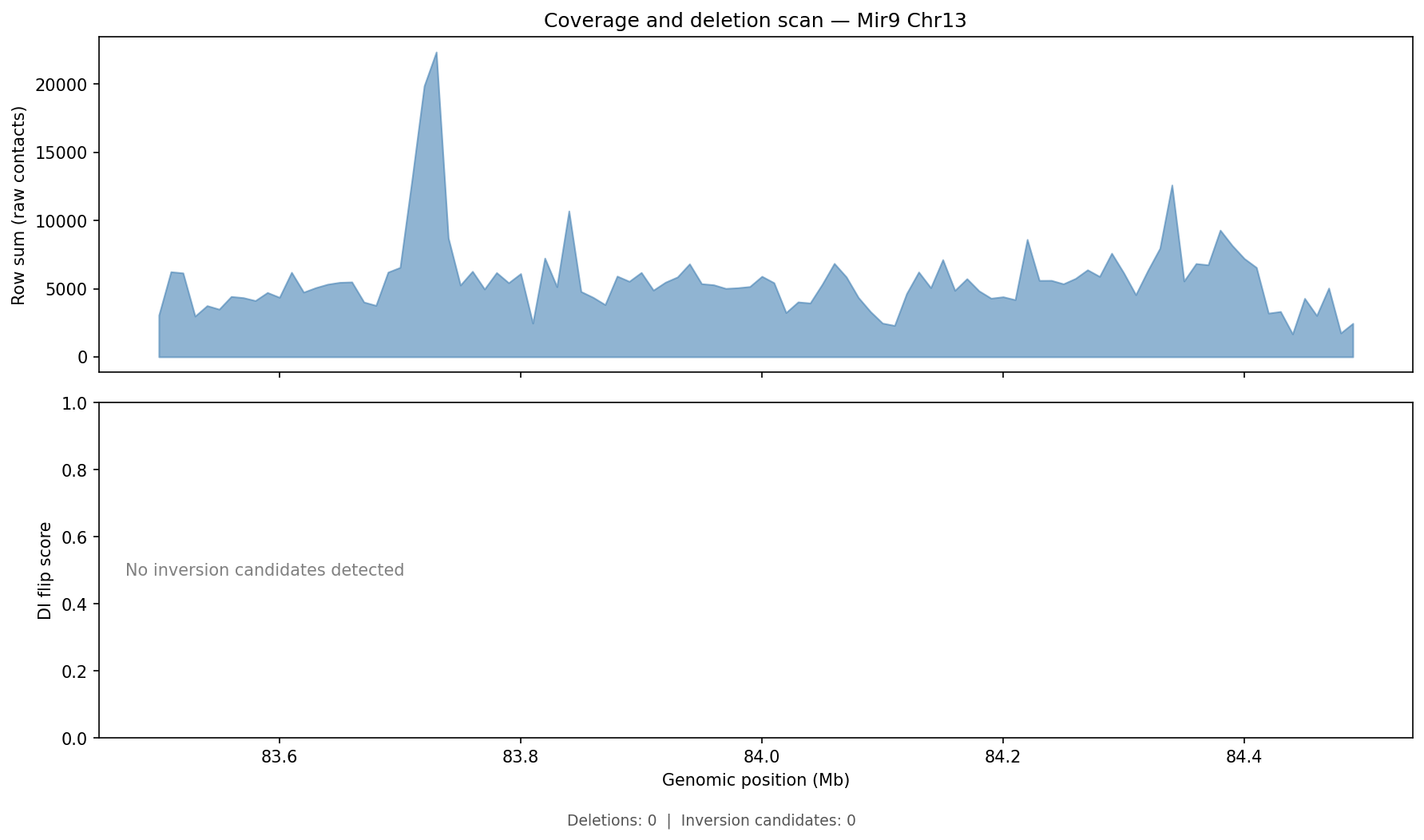
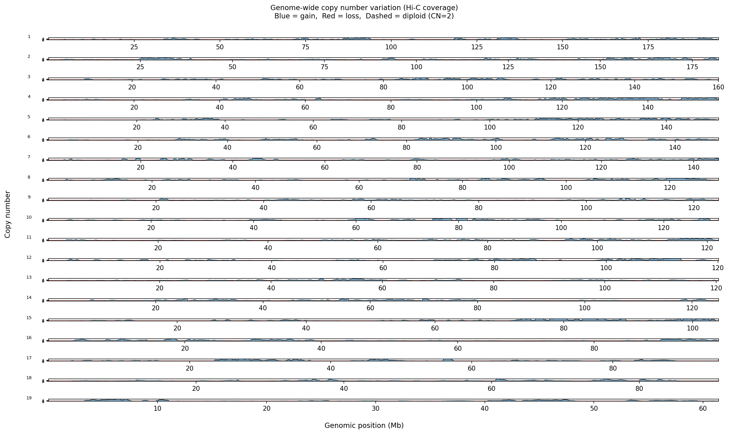
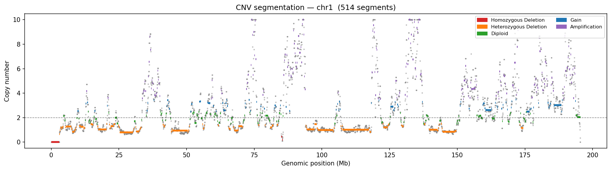
Structural Variant & CNV Detection 50 kb bins

LinkPrep's uniform Tn5-based coverage makes it particularly powerful for SV/CNV detection alongside 3D genome mapping. Translocations appear as inter-chromosomal contact blocks exceeding a z-score threshold (z > 5) relative to the genome-wide inter-chromosomal background. Deletions / inversions are identified as contiguous coverage gaps flanked by bridging read pairs. CNV is derived from per-bin coverage, normalized by the chromosome-wide median and then segmented with Circular Binary Segmentation (CBS). Dovetail recommends a minimum of 50–100 M no-dup pairs for reliable SV/CNV calling at 50 kb resolution.

Translocation Heatmap

Inter-chromosomal contact enrichment across all 19 mouse autosomes at 50 kb. True translocations show focal hotspots; diffuse signal reflects Hi-C background noise.

Deletion Scan — Sox11 chr12

Coverage profile (top) and directionality index flip score (bottom). 0 deletions detected — expected for germline Micro-C data from a normal mouse sample.

Deletion Scan — Mir9-2 chr13

SV scan for the Mir9-2 region. Clean coverage confirms no structural rearrangements at this locus in the public dataset.

Genome-wide CNV

Copy number per chromosome from Hi-C coverage at 50 kb bins. Normal mouse genome shows diploid copy number (CN=2) across all autosomes.

CNV Segments — chr12

Segmented copy number profile for chr12. 514 segments detected. CBS calls stable CN plateaus; color-coded by gain/loss status.

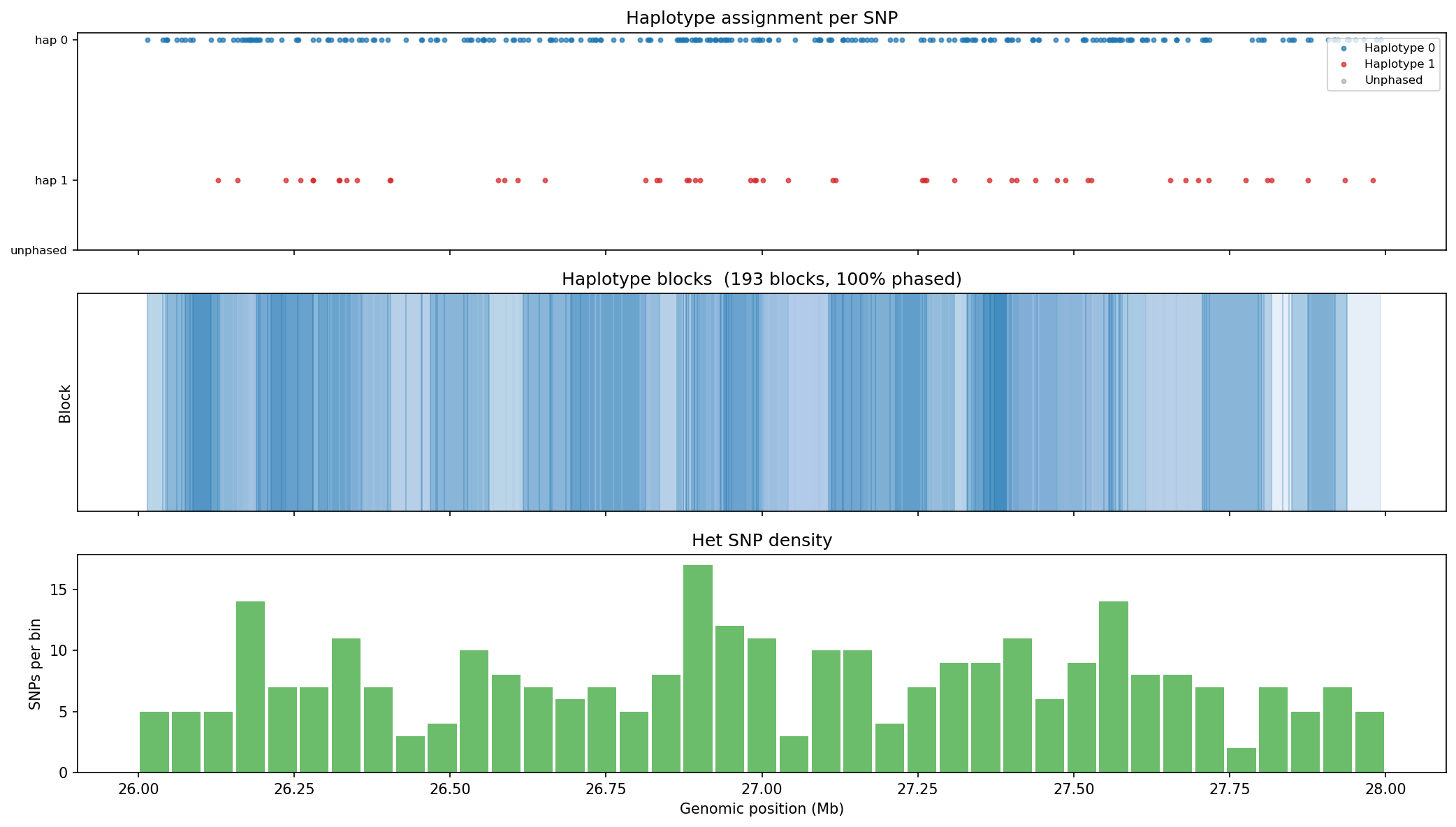
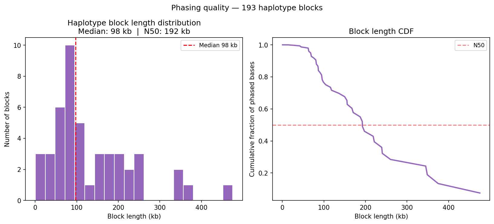
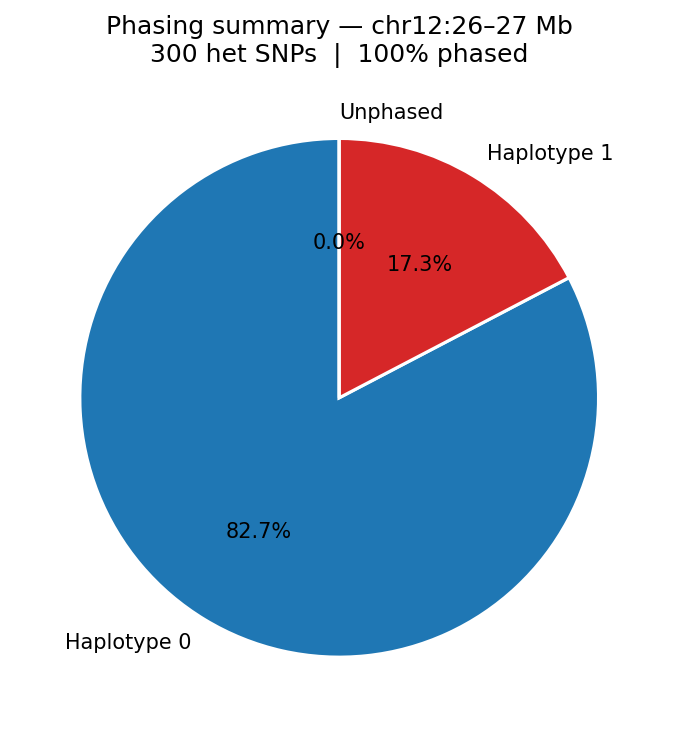
Haplotype Phasing Graph-Based

Hi-C long-range contacts link heterozygous SNPs across megabase distances, enabling chromosome-scale phasing without long reads. Heterozygous SNPs from a VCF are grouped into haplotype blocks using Hi-C read-pair connectivity: two SNPs are placed in the same block if a sufficient number of read pairs span both positions and consistently support the same haplotype assignment (graph-based phasing). Typical N50 for Hi-C phasing is chromosome-scale (Mb range) with sufficient sequencing depth. Input: heterozygous SNPs from VCF + aligned BAM.

Haplotype Block Map

300 het SNPs grouped into 193 haplotype blocks. Each colored bar = one phased block. With real Hi-C data the N50 is typically Mb-scale because long-range pairs link distant SNPs.

Block Length Distribution

Histogram of phasing block lengths with N50 marked. Distribution reflects the density of informative Hi-C read pairs bridging adjacent het SNPs.

SNP Density

Heterozygous SNP density per bin. Uniform density confirms unbiased fragmentation. Gaps indicate low-complexity or repeat-rich regions where variant calling is unreliable.

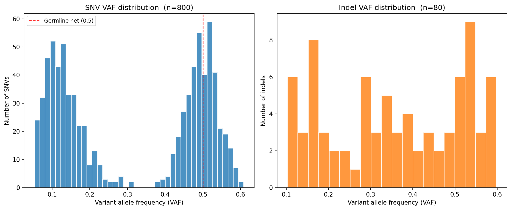
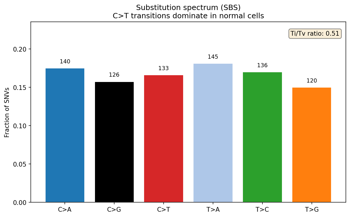
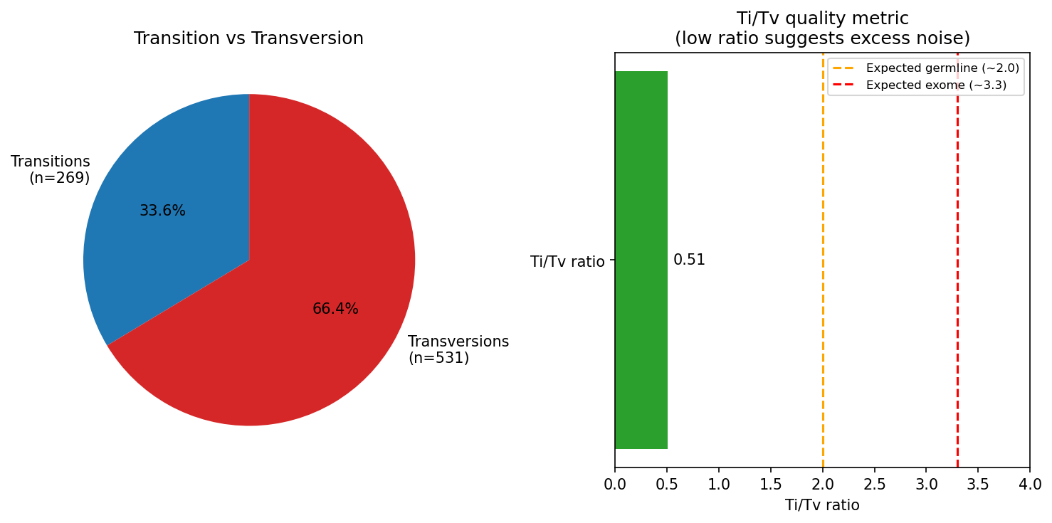
Variant Analysis SNV / Indel

SNV and indel calling from Hi-C-aligned reads. Variant spectrum analysis characterizes mutational signatures: C>T transitions (spontaneous deamination) dominate in normal genomes; APOBEC-driven patterns (C>T/G in TC context) are elevated in certain cancers; UV signature shows C>T at dipyrimidines. Ti/Tv ratio (transition to transversion) is expected ~2.0 genome-wide and ~3.3 in exomes; values below 1.5 suggest sequencing noise or overly relaxed variant filters. Variant allele frequency (VAF) distribution distinguishes germline heterozygous variants (VAF ~0.5) from somatic mosaic variants (VAF 0.05–0.3).

VAF Histogram

Variant allele frequency distribution. Germline het variants cluster at VAF~0.5; somatic mosaic variants appear at low VAF (0.05–0.3). 800 SNVs + 80 indels in the demonstration dataset.

Mutation Spectrum

SBS mutation spectrum showing trinucleotide context. C>T transitions dominate in normal genomes (spontaneous deamination). APOBEC-driven tumors show C>T/G in TC context.

Ti/Tv Ratio

Transition/transversion ratio. Expected ~2.0 genome-wide. Values <1.5 suggest sequencing noise or relaxed filters.

How to Run on Real Data

Activate the hic-analysis conda environment and follow the steps below. The preprocessing script follows the Dovetail recommended parameters exactly. An AlphaGenome API key is required only for visualize_alphagenome.py.

# Prerequisites (Dovetail recommended tools)
conda activate hic-analysis

# Step 1: Preprocess FASTQ → .mcool
# Following Dovetail: BWA-MEM -5SP -T0 | pairtools parse --min-mapq 40
bash scripts/preprocess_microc.sh reference.fa R1.fq.gz R2.fq.gz sample 16

# Step 2: Run QC (Dovetail get_qc.py compatible metrics)
# Threshold: cis ≥1kb > 40% of no-dup reads
python -c "import cooler; clr = cooler.Cooler('sample.mcool::resolutions/5000'); print(clr.info)"

# Step 3: Run all analyses
python visualize_compartments.py   # 25 kb, E1 eigenvector
python visualize_loops.py          # 5 kb, donut background model
python analyze_hichip.py           # HiChIP, requires ChIP-seq peaks BED
python analyze_capture_hic.py      # Capture Hi-C, requires baits BED
python analyze_sv_cnv.py           # 50 kb, genome-wide
python analyze_phasing.py          # Requires het SNP VCF
python analyze_variants.py         # Requires variant VCF