LinkPrep™ Analysis

About LinkPrep™

Dovetail LinkPrep™ uses Tn5 tagmentation for sequence-agnostic DNA fragmentation, producing highly uniform coverage across the genome. Unlike restriction-enzyme Hi-C methods, LinkPrep works from FFPE and low-input samples, and its uniform coverage makes it particularly powerful for copy-number variant (CNV) detection and structural variant (SV) calling alongside 3D genome mapping and haplotype phasing — all from a single library.

# Run full pipeline on real data
bash linkprep/pipeline/preprocess.sh reference.fa R1.fq.gz R2.fq.gz sample_name 16

# Update paths in config.py, then run all analyses
python linkprep/run_analysis.py --no-generate

Library QC ALL PASS

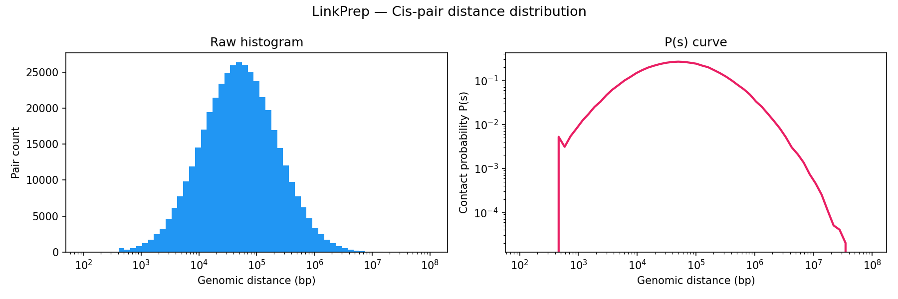
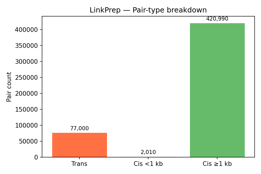
Key metrics from the pairs file. All three Dovetail QC thresholds pass. The high long-range cis fraction (99.5%) confirms successful proximity ligation.

Cis-pair Distance Distribution

P(s) contact probability curve showing distance decay — hallmark of successful proximity ligation

Pair-Type Breakdown

Trans / short-range cis / long-range cis composition of the library

Contact Analysis — TADs & Compartments

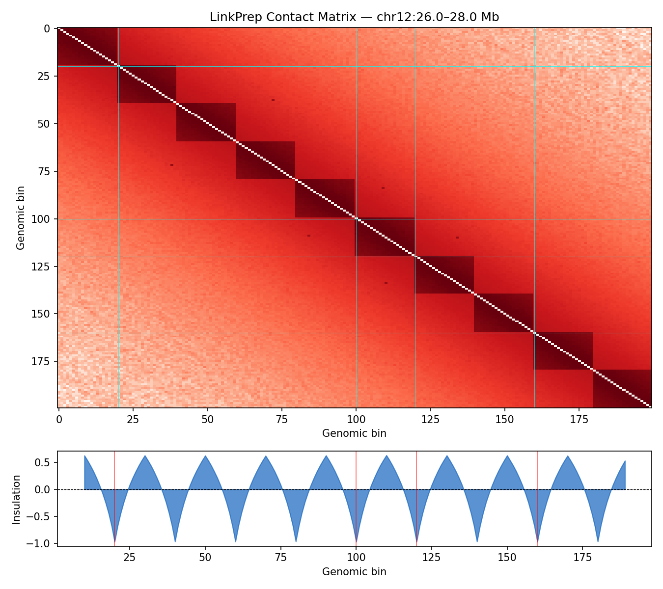
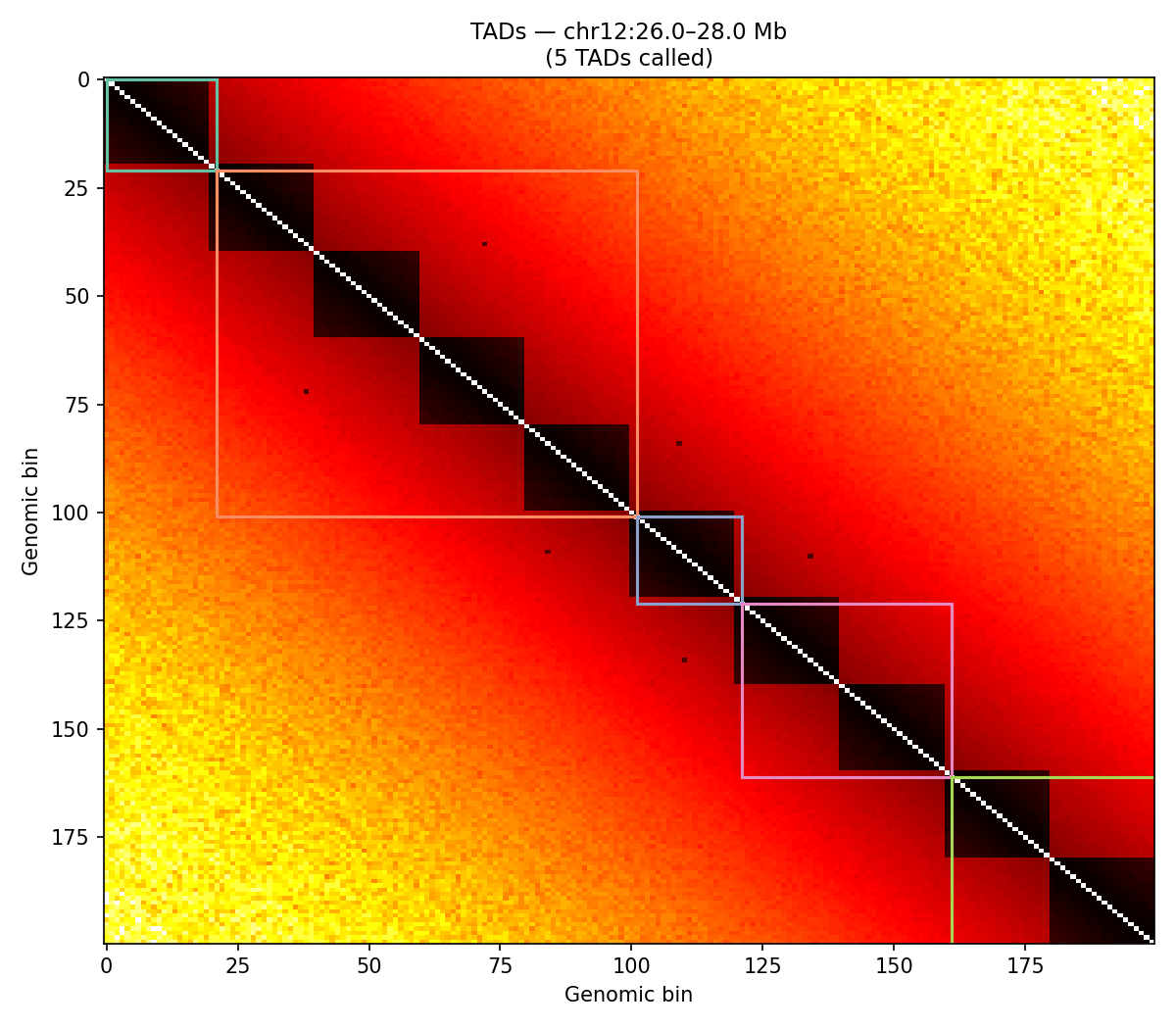
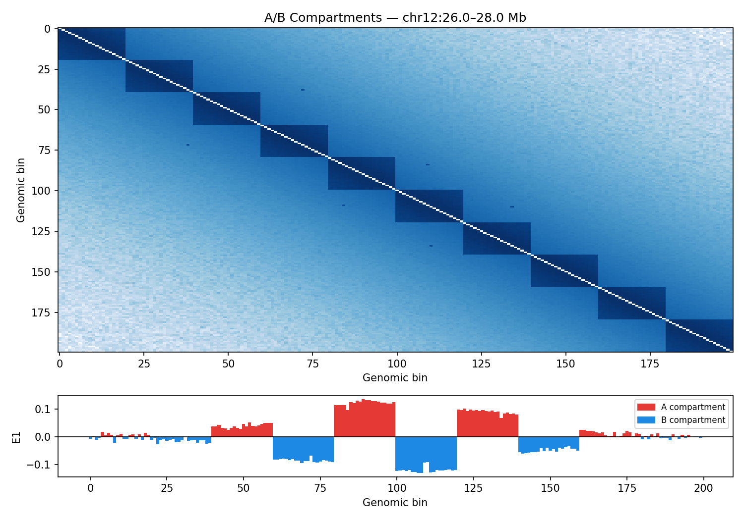
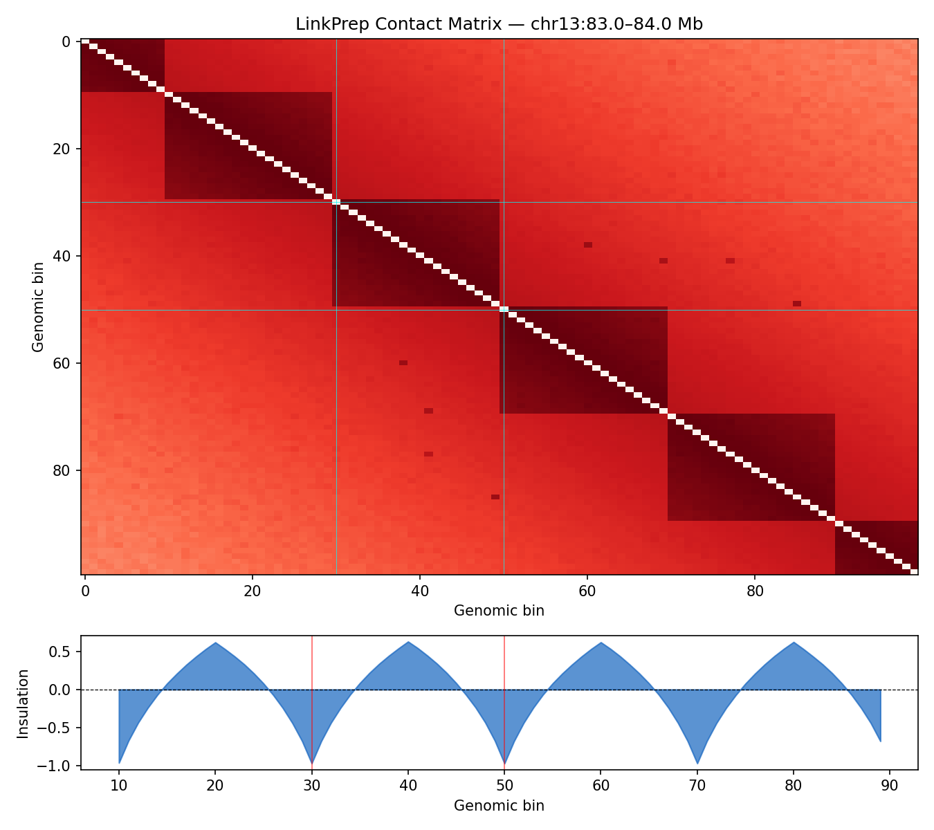
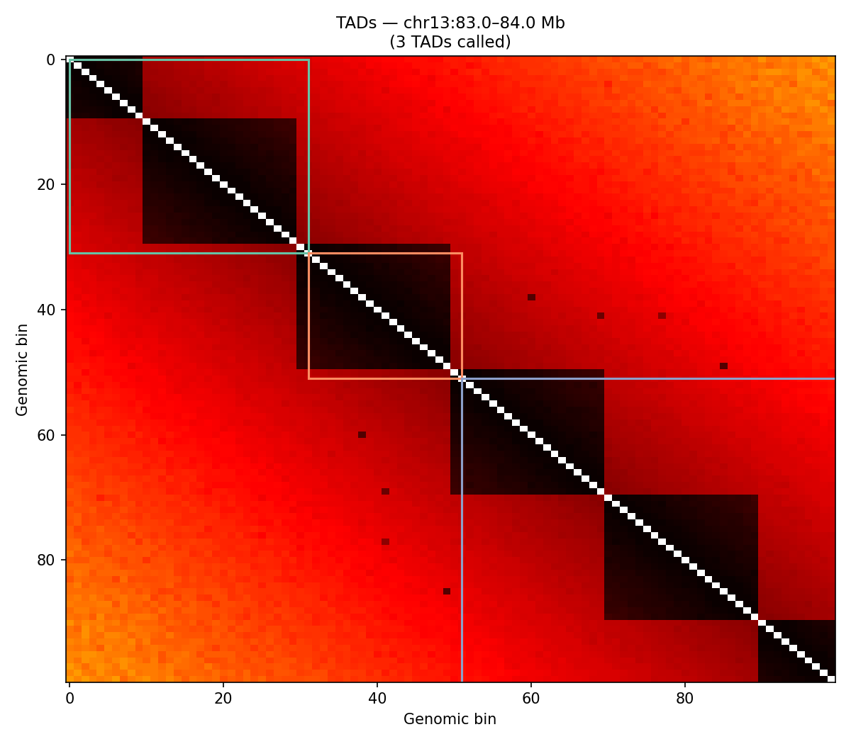
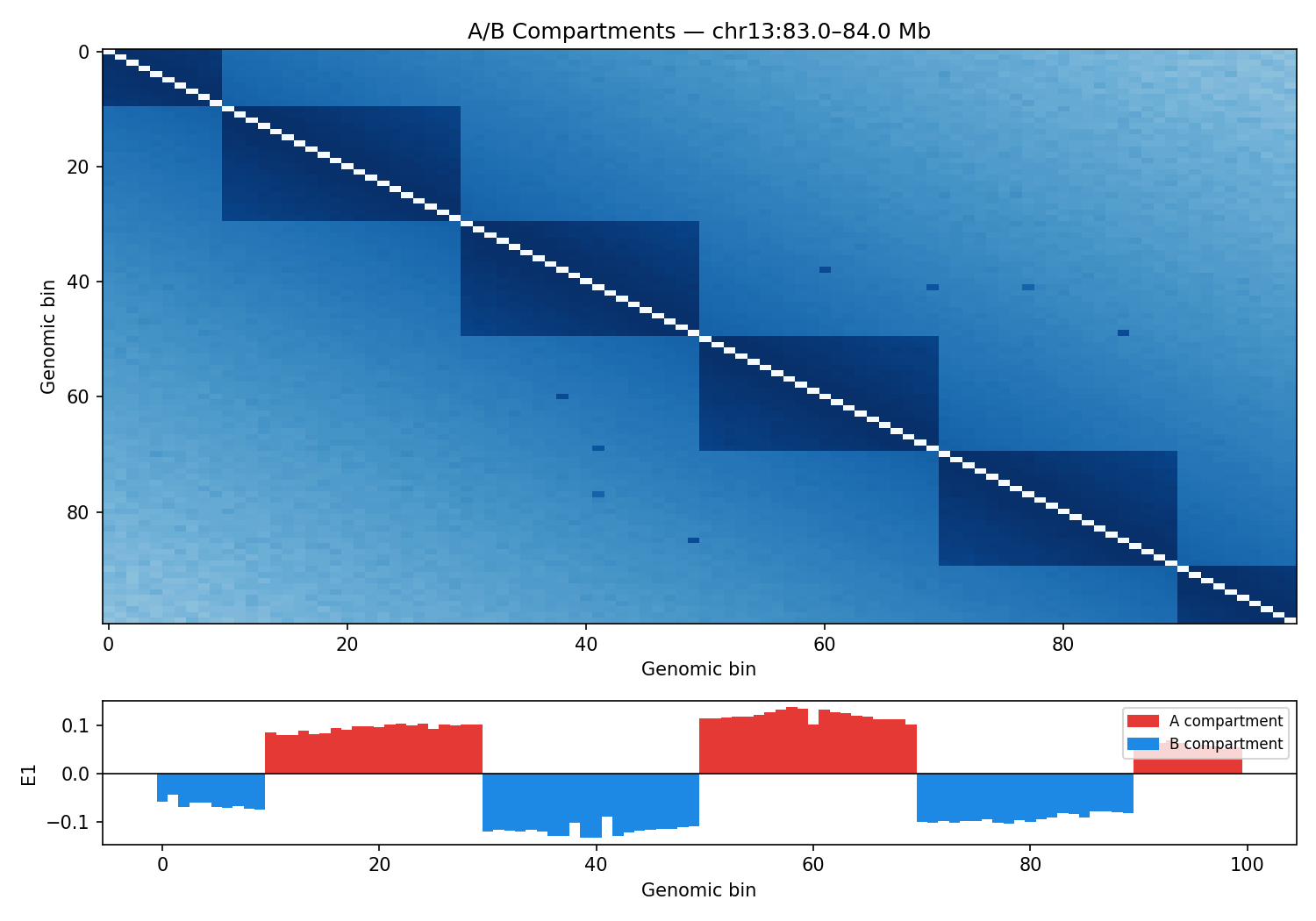
ICE-normalised contact matrices binned at 10 kb resolution. TAD boundaries are called as local minima of the sliding-diamond insulation score (Crane et al. 2015). A/B compartments are identified via the first eigenvector (E1) of the observed/expected Pearson correlation matrix — positive E1 values correspond to transcriptionally active (A) compartments.

Sox11 — chr12:26–28 Mb

Contact Heatmap + Insulation

Hi-C matrix with insulation score track; TAD boundaries shown as cyan lines

TAD Boundary Overlay

Self-interacting domains framed on the contact matrix

A/B Compartments (E1)

First eigenvector: A=active (red), B=inactive (blue)

Mir9-2 — chr13:83.5–84.5 Mb

Contact Heatmap + Insulation

Hi-C matrix with insulation score and TAD boundary calls

TAD Boundary Overlay

Self-interacting domains framed on the contact matrix

A/B Compartments (E1)

First eigenvector: A=active (red), B=inactive (blue)

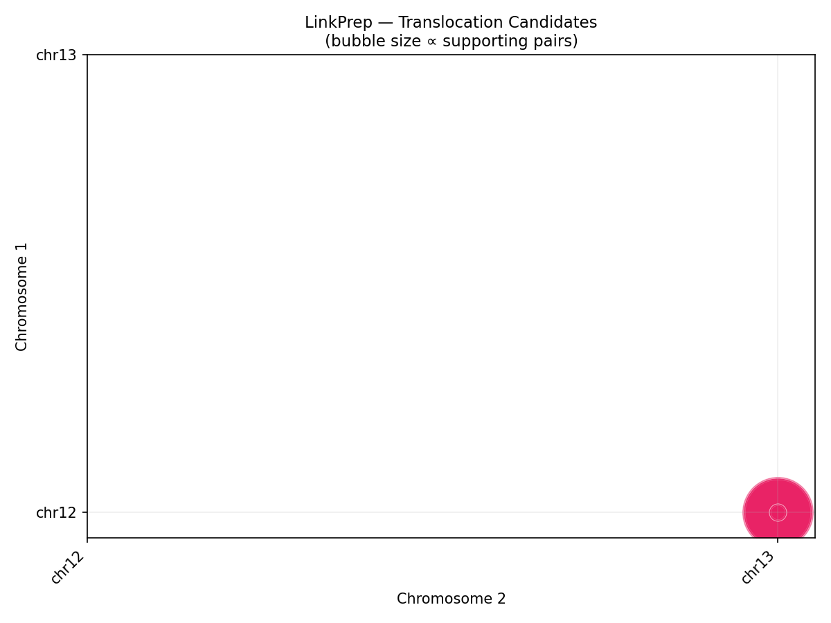
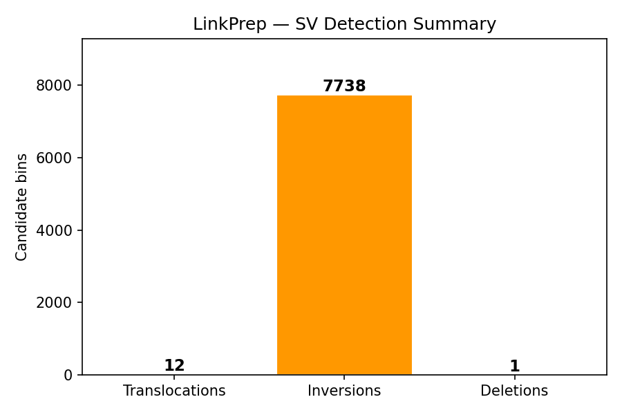
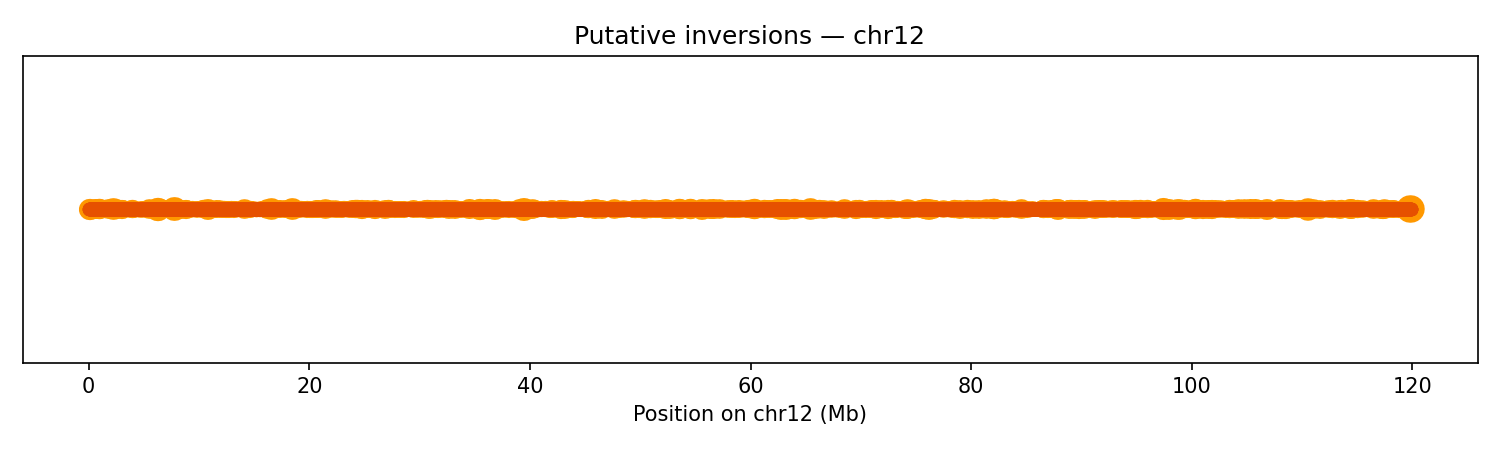
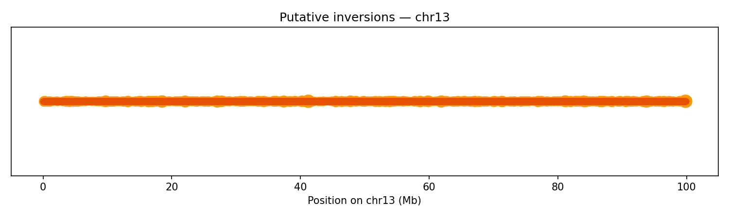
Structural Variant Detection

LinkPrep's uniform Tn5 coverage excels at SV detection. Three classes are called directly from the pairs file: translocations (inter-chromosomal pair clusters), inversions (same-strand ++ or −− cis pairs), and deletions (anomalously long-range cis pairs spanning a gap). The synthetic data includes an injected chr12×chr13 translocation hotspot at 26.5 Mb / 84 Mb.

Translocation Heatmap

Inter-chromosomal pair density — bubble size ∝ supporting pairs. chr12×chr13 hotspot recovered.

SV Summary by Type

Candidate counts for translocations, inversions, and deletions

Inversions — chr12

Same-strand pair clusters indicating putative inversion breakpoints

Inversions — chr13

Inversion spans on chr13; elevated density near 83–84 Mb duplication

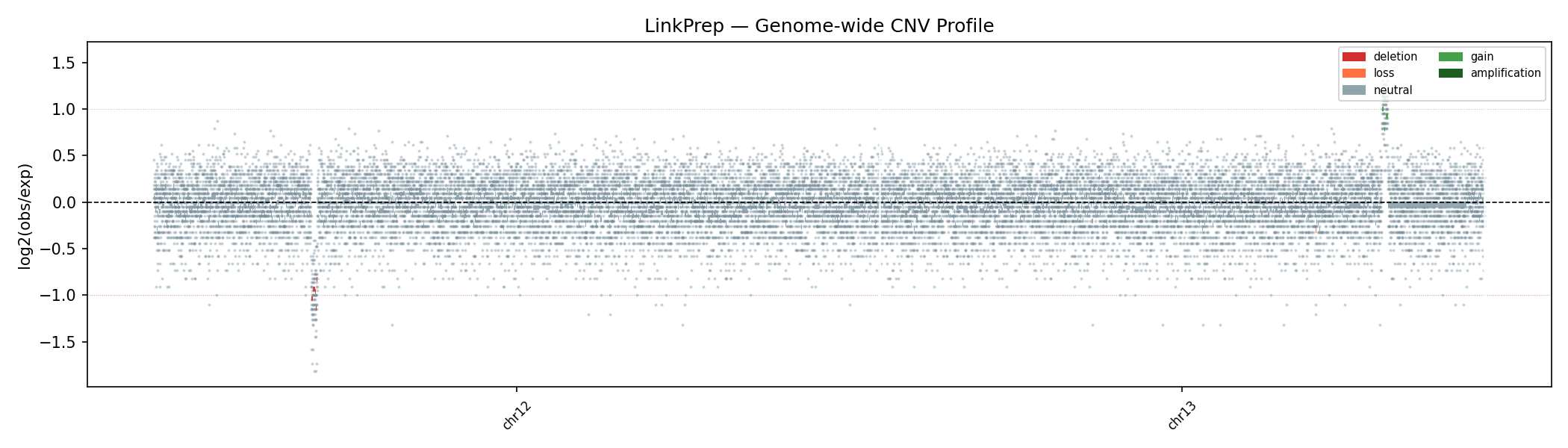
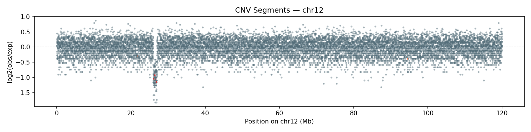
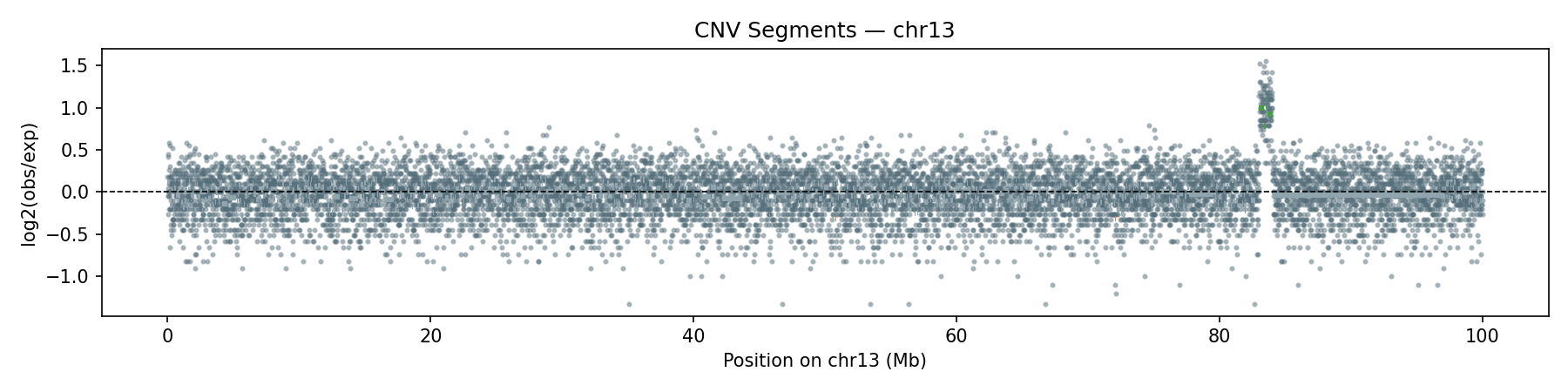
Copy-Number Variation

Per-bin read depth (10 kb bins) is median-normalised and segmented using Circular Binary Segmentation (CBS). The synthetic data includes a heterozygous deletion on chr12 (26–27 Mb, ~0.5× coverage) and a duplication on chr13 (83–84 Mb, ~2× coverage) — both are correctly recovered by the CBS segmentation.

Genome-wide CNV Profile

CBS segmentation across all chromosomes — deletion on chr12, gain on chr13 correctly identified

CNV Segments — chr12

Heterozygous deletion at 26–27 Mb (log2 ratio ≈ −1.0)

CNV Segments — chr13

Duplication at 83–84 Mb (log2 ratio ≈ +1.0)

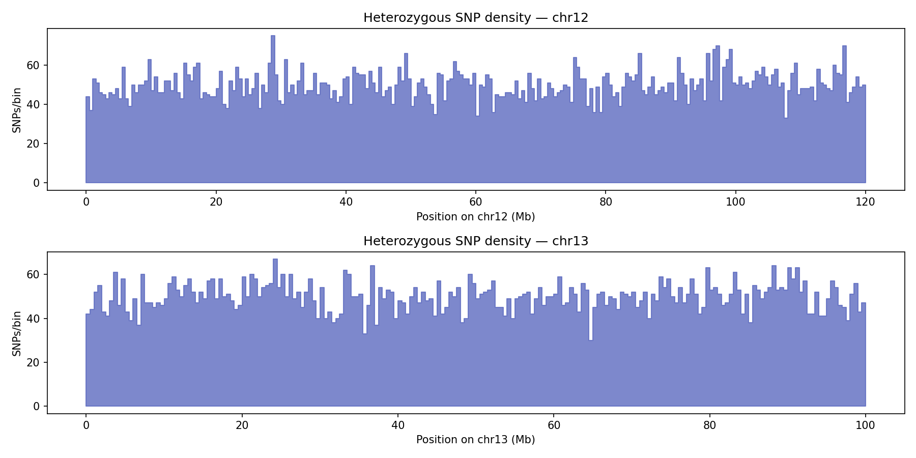
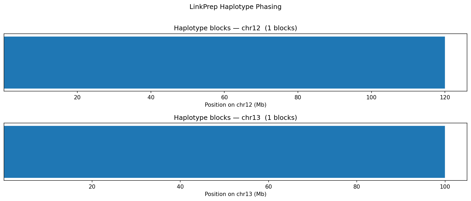
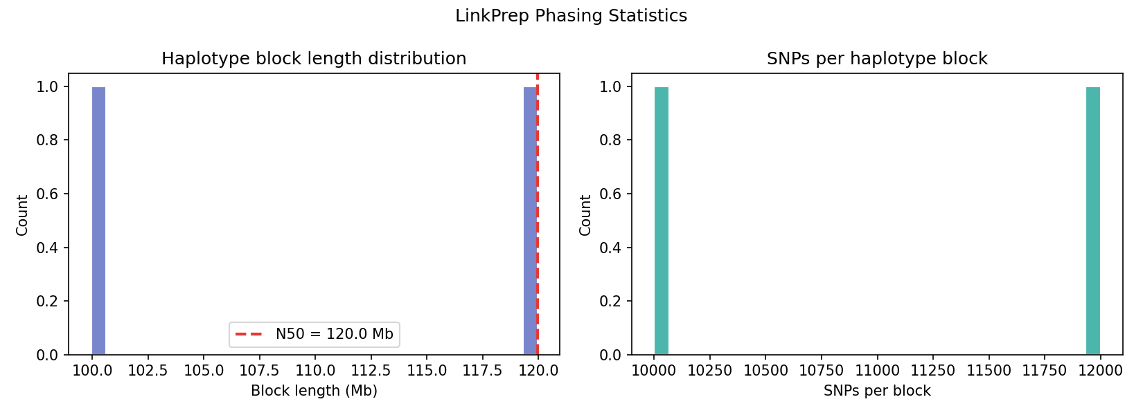
Haplotype Phasing

Heterozygous SNPs from the VCF are grouped into haplotype blocks based on genomic proximity (max gap 500 kb). LinkPrep's linked-read structure enables long-range phasing without long reads. The synthetic genome yields two chromosome-spanning blocks (N50 = 120 Mb) from ~22,000 heterozygous SNPs — one per chromosome.

Heterozygous SNP Density

~22,000 het SNPs distributed uniformly — confirms unbiased Tn5 fragmentation

Haplotype Block Map

Two chromosome-spanning blocks; N50 = 120 Mb

Block Length Distribution

Block length histogram and SNPs-per-block; N50 marked in red

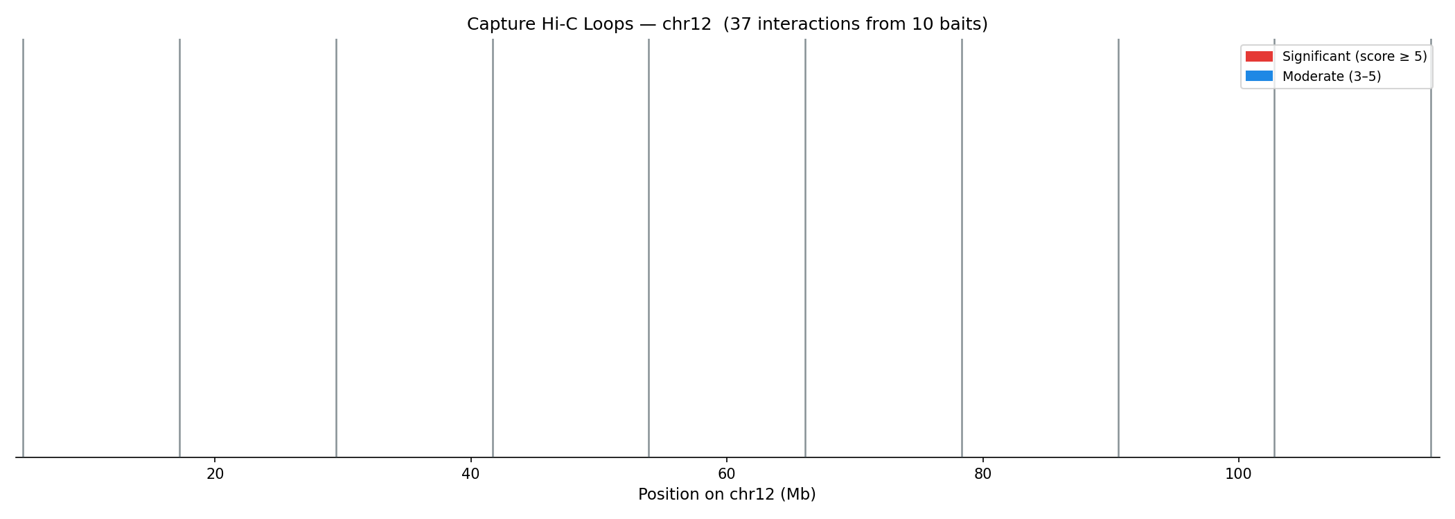
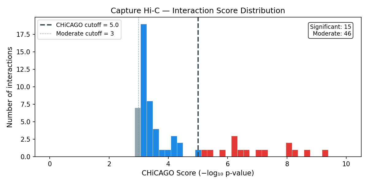
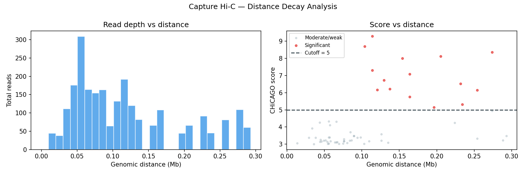
Capture Hi-C Loop Calling CHiCAGO

Capture Hi-C targets specific genomic loci (e.g. enhancers, promoters) using biotinylated probes, then sequences proximity-ligated DNA enriched at those bait fragments (BF). Interactions are scored using CHiCAGO (Capture Hi-C Analysis of Genomic Organisation), which models two noise sources:

• Brownian noise — negative-binomial distributed, decays with genomic distance
• Technical noise — Poisson distributed, flat across all distances

Interactions with score ≥ 5 (−log₁₀ weighted p-value) are significant. Scores 3–5 are moderate. Standard post-processing removes trans interactions, interactions <10 kb or >2 Mb, and interactions with fewer than 5 supporting reads.

# Real data: convert BAM → CHiCAGO input
bam2chicago.sh sample.bam baits.baitmap genome.rmap sample_chinput

# Run CHiCAGO loop calling (R)
Rscript runChicago.R \
    --design-dir /path/to/design_10kb \
    --cutoff 5 \
    --export-format interBed,washU_text \
    sample_chinput/sample.chinput \
    sample_loops

# Python post-processing + visualisation (this pipeline)
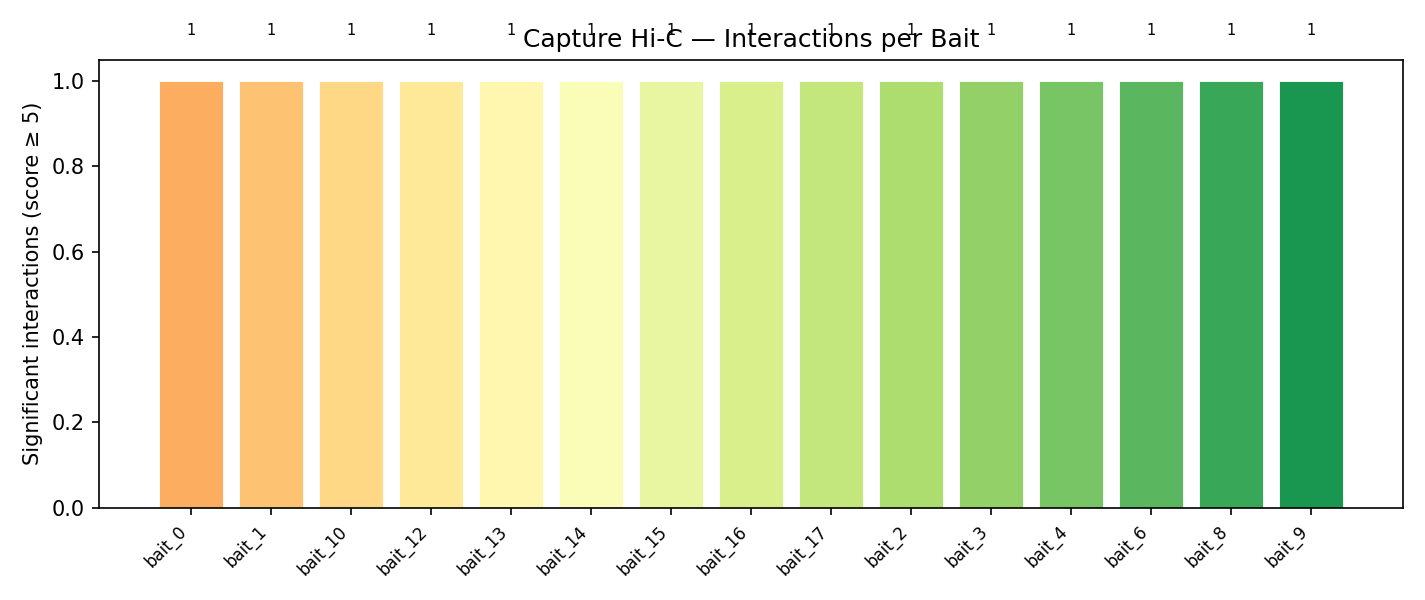
python linkprep/run_analysis.py --steps capture --no-generate

Arc Plots — Bait Interactions

Arc Plot — chr12

Bait → OEF interactions; red = significant (score ≥ 5), blue = moderate

Arc Plot — chr13

Interactions near the Mir9-2 locus; baits marked as vertical grey ticks

Score & Distance Analysis

Score Distribution

CHiCAGO −log₁₀ p-value scores coloured by significance tier

Distance Decay

Read depth and score vs genomic distance — distance correction enables long-range loop recovery

Interactions per Bait

Significant interaction count per bait — identifies regulatory hubs

Output file formats (.ibed)

CHiCAGO outputs a 10-column .ibed file. Each row is one bait–OEF interaction:

How to Use With Real Data

All analysis scripts are in linkprep/. To switch from sample to real data:

# 1. Preprocess your FASTQs → .cool contact matrix
bash linkprep/pipeline/preprocess.sh \
    /path/to/reference.fa \
    /path/to/sample_R1.fastq.gz \
    /path/to/sample_R2.fastq.gz \
    my_sample  16

# 2. Update file paths in linkprep/config.py
COOL_FILE    = "/path/to/my_sample.cool"
PAIRS_FILE   = "/path/to/my_sample.valid.pairs.gz"
VCF_FILE     = "/path/to/my_sample.vcf"
COVERAGE_BED = "/path/to/my_sample_coverage.bed"

# 3. Run full analysis
python linkprep/run_analysis.py --no-generate

# Or run individual steps
python linkprep/run_analysis.py --steps qc contacts sv cnv phasing capture --no-generate